I developed some Matlab code to generate high-quality 3D animated visualizations of the magnetic field outside the UMD Three Meter Geodynamo Experiment. An analytical representation of the field everywhere outside the sphere was obtained by fitting suitable vector spherical harmonics to the measurements from an array of 31 Hall-effect sensors outside the outer sphere.
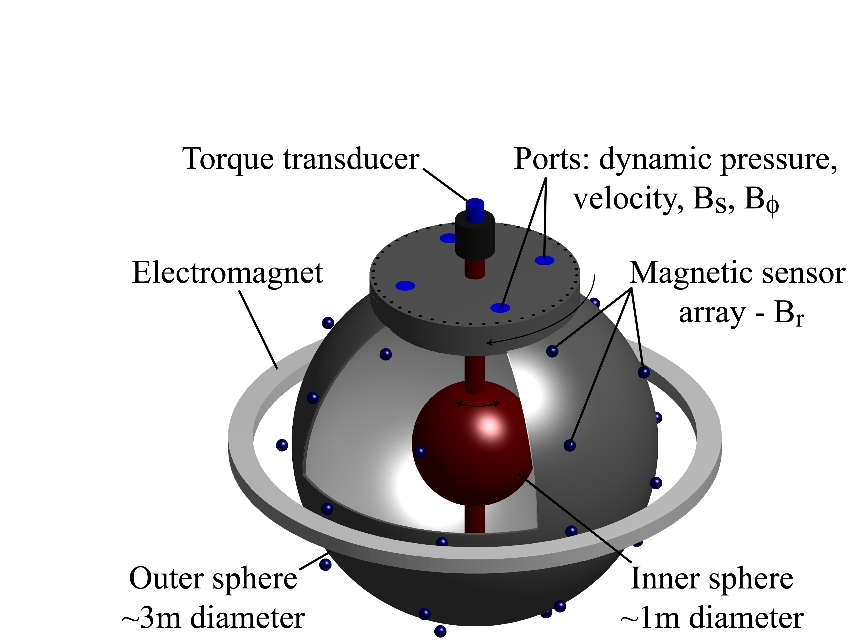
Sensors and reconstructed external field snapshot from the 3m experiment
To draw field lines, a collection of initial points are chosen in the space around the sphere, and each point is swept through space as if the magnetic field were a velocity field. The resulting trajectories of the test points are magnetic field lines:
Animated example of magnetic field "trajectory" calculation
The code that calculates the field lines from vector spherical harmonic fits to the probe data is optimized, vectorized Matlab code that simultaneously calculates the trajectories of an array of points. My code uses an Euler predictor-corrector method to integrate the trajectories of the test points. I started with a simple Euler integrator, but the error growth was rapid enough to give visually poor results in some cases. This was especially noticeable when integrating in test fields with simple structure, and the predictor-corrector scheme greatly improved it.
The calculations are accelerated by marking and tracking inactive field lines.
When individual trajectories reach a predetermined external radial boundary or the surface of the outer sphere,
they're marked as terminated with a NaN, and they are no longer tracked or calculated. This speeds up the calculation
significantly when many field lines are computed, and it makes sure that lines don't loop into and back out of the sphere's surface.
The NaN-padding throughout the resulting array of trajectory data is conveniently ignored by
Matlab when trajectories are plotted.
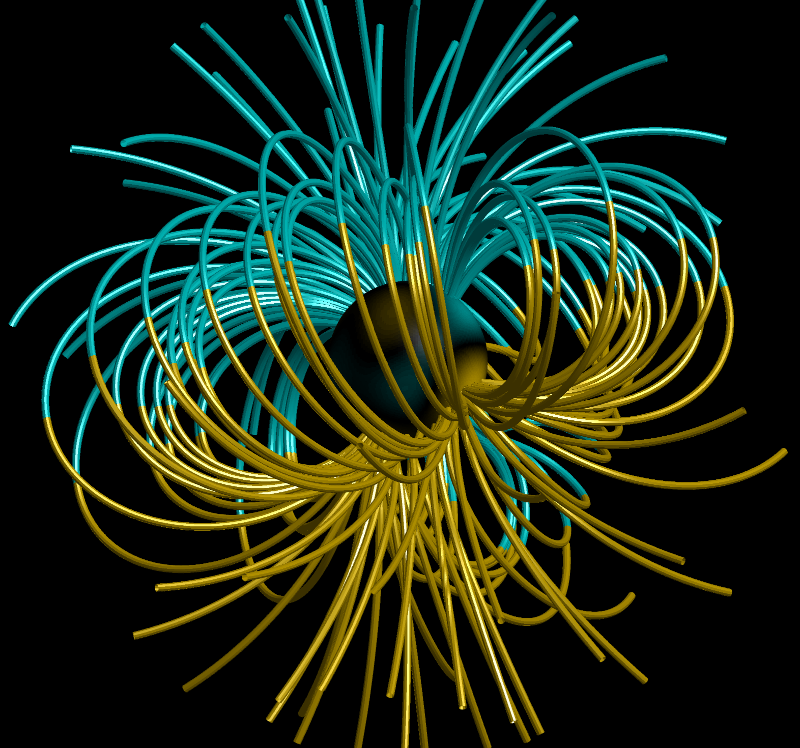
After the field lines are computed for each frame, they are plotted as 3D tubes using the nice library available at http://www.aleph.se/Nada/Ray/Tubeplot/tubeplot.html. A color plot of field intensity on the outer sphere surface is also included. Some extra lighting and other features finish off the look. The codebase is some serious academic spaghetti, and I haven't found the time to clean it up, but it's available on Github if you want to take a look:
Final Product
There's some art to making nice animations of a time-varying vector field like this. I used a couple clever methods to achieve the smoothly drifting and nicely bundled field lines seen in the movie below. First of all, the field lines are initialized on a regularly spaced spherical grid in the space further away from the sphere. They're integrated in both directions and those that approach the sphere naturally bundle into the strong field areas there. This makes the lines emerge preferentially in dense bundles from the strong surface patches.
I also initialized the initial seed points with a rotating drift that matches the drift speed of the dominant field shape. In movies with a single-frequency drifting wave, I used a constant-speed rotating drift. This works well for some cases. Eventually, I started using the instantaneous drift speed as a function of time computed from the rate of change of the azimuthal phase angle of the strongest field components. This gives superior results in results like the movie above, where the dominant drift is not always well described by a progressive azimuthal rotation.